First Sensor Data Log Test Run

At this point in the project, most of the sensors were finally in place.

That included:

Brake disc temperature sensors
Tyre temperature sensors
GPS data from the rear section
Suspension movement using ultrasonic ranging
Engine coolant temperature
Input sensing from the front brake, rear brake, and headlight switch

With all of that hardware installed and communicating, it was finally time to answer a simple question:

What does the data actually look like when you ride the bike?

How the system was powered and networked

Before getting into the data itself, it’s important to explain how everything was running during the test ride, because this setup played a big role in how stable the system turned out to be.

All sensor modules were powered from a single 5V power rail, supplied by a separate power bank. This was a deliberate design choice. I wanted the entire sensing and logging system to be electrically isolated from the bike’s main electrical system.

That isolation had a few advantages:

No risk of interfering with the bike’s ECU or wiring
Reduced electrical noise from the bike
Easier debugging when something went wrong

Once the power bank was switched on, all sensor modules booted automatically.

Because the system was fully wireless:

My phone acted as a WiFi hotspot
The phone was also running the data logging engine
All sensor modules connected directly to the phone

This effectively turned the phone into the central hub of the system, handling networking, data collection, and storage at the same time.

In practice, this setup worked surprisingly well. All sensors were within range of the phone, and I never experienced WiFi dropouts during the ride. Every module stayed connected and streamed data continuously.

Looking back, isolating power and keeping networking simple probably saved me from a lot of intermittent and hard-to-debug problems.

The first real data logging run

The first test run itself wasn’t anything extreme. It was simply a ride from home to my workplace under normal riding conditions.

At the time, I wasn’t entirely sure how I would handle the data once it came in. I had already written multiple versions of a Python-based logging engine, and the earlier versions stored data in CSV format.

That’s what I used for the first run.

The ride went smoothly. The sensors logged. The system didn’t crash.

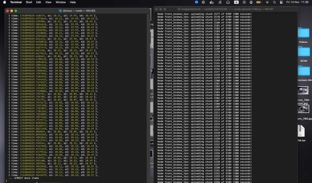
Then I opened the data file.

Realizing the data was too large to handle locally

The CSV file was massive.

There was no realistic way to:

Scroll through it comfortably
Inspect it manually
Make sense of it directly on my laptop

That’s when I started thinking about moving the analysis somewhere with more computing power.

The obvious answer was the cloud.

A quick and messy data pipeline (that still worked)

The workflow I came up with wasn’t elegant, but it got the job done:

Convert the CSV data into JSON
Upload the converted data to Firebase
Load the data into Google Colab
Explore and visualize it using Python

I honestly don’t remember why Firebase was the first thing that came to mind, but it worked.

The downside was obvious:

Conversion took time
Uploading the large dataset was slow
The workflow felt fragile and unsustainable

Still, once the data was available in Google Colab, I could start exploring.

Seeing the data for the first time

This was the moment where everything started to feel real.

Inside Google Colab, I loaded the dataset and began plotting different signals:

Brake disc temperature over time
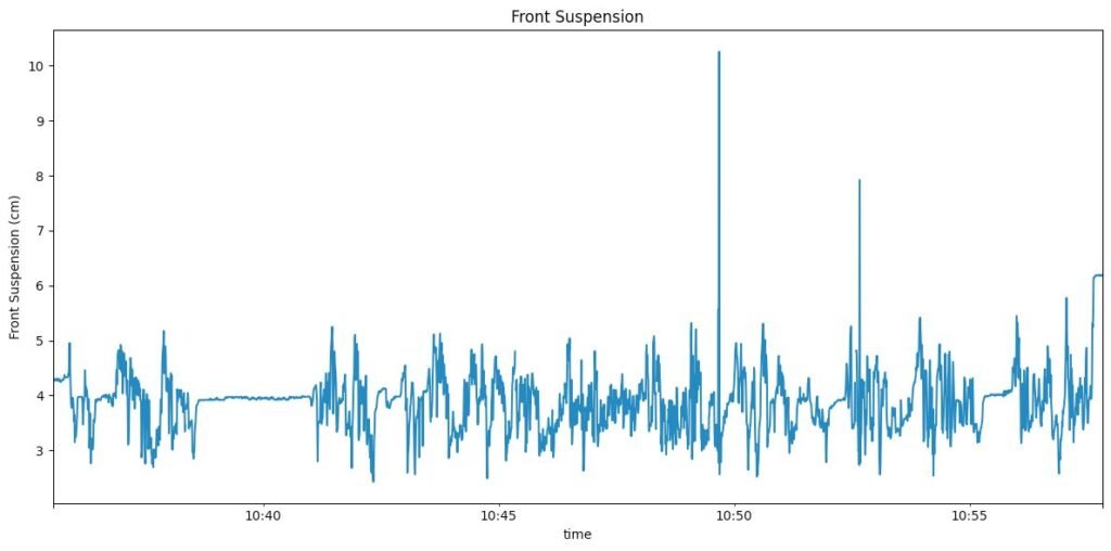
Suspension movement during braking
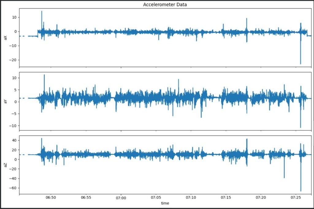
Responses during acceleration
General trends across the ride

Nothing fancy—mostly basic plotting using pandas and matplotlib, tools I had only lightly touched back in college.

But seeing data generated by hardware I built, from a bike I rode, plotted in front of me was incredibly satisfying.

Discovering a major flaw: time synchronization

As exciting as it was, something didn’t look right.

I noticed that:

Different sensors produced different numbers of data frames
Some data streams were much denser than others
Events didn’t line up cleanly across sensors

Up until this point, I had made a bad assumption.

I assumed that because all sensor modules booted at roughly the same time, their data would naturally be synchronized.

That wasn’t true.

Some modules:

Ran faster loops
Had more processing overhead
Sent data at different rates

There was no shared clock.

Rethinking the logging approach

This forced me to rethink how the logging engine worked.

Two ideas came up:

Time-slot based logging

Instead of logging whenever data arrived, I could:

Define a fixed time window (for example, once per second)
Sample the latest values from all sensors
Store them together as a single frame

This would force alignment.

Switching to JSONL

Instead of CSV → JSON conversion, I could:

Log directly as JSON Lines (JSONL)
Append one structured record per time slot
Upload a single file
Load it directly into Google Colab

We tried this approach—and it worked far better.

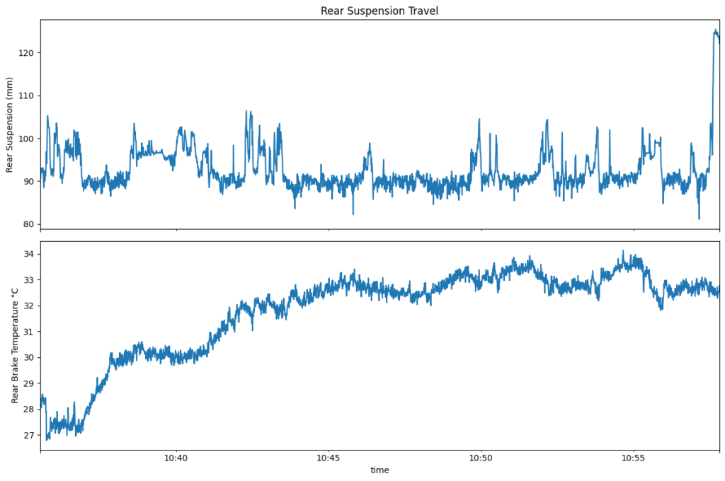
When everything finally lined up

Once the data was time-aligned, everything clicked.

Now I could clearly see:

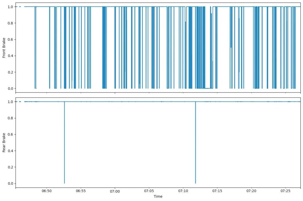
Brake input events
Immediate suspension response
Brake disc temperature rising
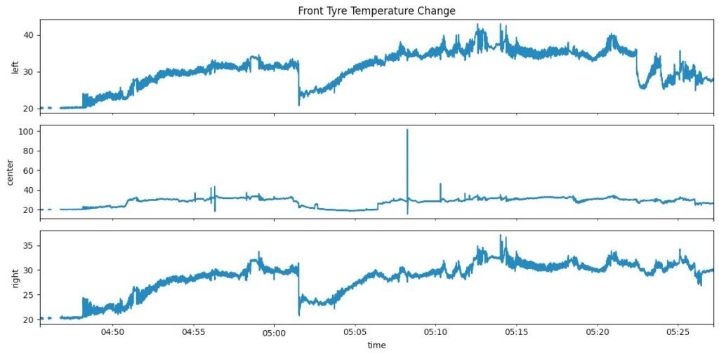
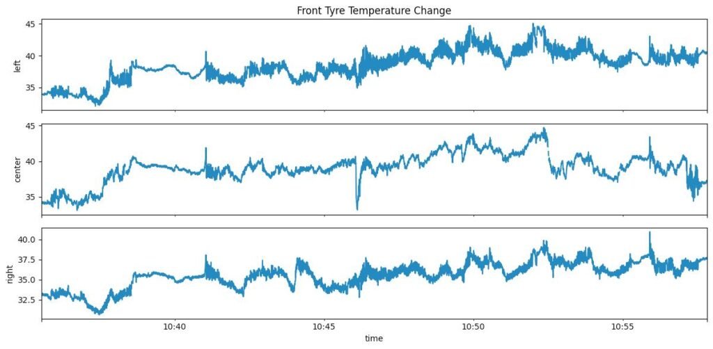
Tyre temperature reacting more slowly

I could brake hard and watch the system respond:

Brake signal toggled
Suspension compressed
Brake disc temperature climbed

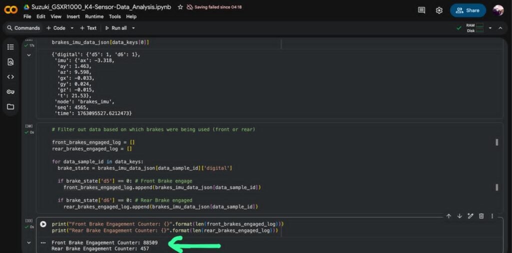
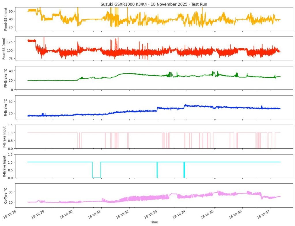
These are some the plots from when I was looking at the data in segments like I could plot the temperature data or IMU data. There is also a brake input plot which are just binary , 1 for when the brake is not engaged and 0 for when the brake is engaged.